circpacker package

Submodules

circpacker.basegeom module

Module to define the Triangle, Circle and Polygon classes. Some properties related to the geometry of these classes are determined. These classes are the basic inputs to pack circular particles in a closed polygon in \(\mathbb{R}^2\).

class circpacker.basegeom.Circle(center, radius)

Bases: object

Creates an instance of an object that defines a Circle once the cartesian coordinates of its center and the radius are given.

center

(x, y)-cartesian coordinates of circle center.

Type:tuple or list

radius

Length of the segment that joins the center with any point of the circumference.

Type:float or int

Examples

>>> center, radius = (0, 0), 1
>>> circle = Circle(center, radius)
>>> circle.__dict__
{'area': 3.141592653589793,
 'center': array([0, 0]),
 'curvature': 1.0,
 'diameter': 2,
 'perimeter': 6.283185307179586,
 'radius': 1}

>>> center, radius = (2, 5), 2.5
>>> circle = Circle(center, radius)
>>> circle.__dict__
{'area': 19.634954084936208,
'center': array([2, 5]),
'curvature': 0.4,
'diameter': 5.0,
'perimeter': 15.707963267948966,
'radius': 2.5}

Note

The class Circle requires NumPy

descartesTheorem(circle1, circle2=None)

Method to determine the tangent circles of the Descartes theorem.

To find centers of these circles, it calculates the intersection points of two circles by using the construction of triangles, proposed by Paul Bourke, 1997.

Parameters:

circle1 (circle object): Tangent circle to the circle object intantiated. circle2 (circle object): Tangent circle to the circle object intantiated and to the circle1.

Returns:Each element of the tuple is a circle object. Return type:circles (tuple)

Examples

>>> import matplotlib.pyplot as plt
>>> from basegeom import Circle
>>> # Special case Descartes' Theorem (cicle with infite radius)
>>> circle = Circle((4.405957, 2.67671461), 0.8692056336001268)
>>> circle1 = Circle((3.22694724, 2.10008003), 0.4432620600509628)
>>> c2, c3 = circle.descartesTheorem(circle1)
>>> # plotting
>>> plt.axes()
>>> plt.gca().add_patch(plt.Circle(circle.center,
                        circle.radius, fill=False))
>>> plt.gca().add_patch(plt.Circle(circle1.center,
                        circle1.radius, fill=False))
>>> plt.gca().add_patch(plt.Circle(c2.center,
                        c2.radius, fc='r'))
>>> plt.gca().add_patch(plt.Circle(c3.center,
                        c3.radius, fc='r'))
>>> plt.axis('equal')
>>> plt.show()

>>> import matplotlib.pyplot as plt
>>> from basegeom import Circle
>>> # General case Descartes Theorem (three circle tangent mutually)
>>> circle = Circle((4.405957, 2.67671461), 0.8692056336001268)
>>> circle1 = Circle((3.22694724, 2.10008003), 0.4432620600509628)
>>> circle2 = Circle((3.77641134, 1.87408749), 0.1508620255299397)
>>> c3, c4 = circle.descartesTheorem(circle1, circle2)
>>> # plotting
>>> plt.axes()
>>> plt.gca().add_patch(plt.Circle(circle.center,
                        circle.radius, fill=False))
>>> plt.gca().add_patch(plt.Circle(circle1.center,
                        circle1.radius, fill=False))
>>> plt.gca().add_patch(plt.Circle(circle2.center,
                        circle2.radius, fill=False))
>>> plt.gca().add_patch(plt.Circle(c3.center,
                        c3.radius, fc='r'))
>>> plt.axis('equal')
>>> plt.show()

class circpacker.basegeom.Triangle(coordinates)

Bases: object

Creates an instance of an object that defines a Triangle once the coordinates of its three vertices in cartesian \(\mathbb{R}^2\) space are given.

It considers the usual notation for the triangle ABC in which A, B and C represent the vertices and a, b, c are the lengths of the segments BC, CA and AB respectively.

coordinates

Coordinates of three vertices of the triangle.

Type:(3, 2) numpy.ndarray

Note

The class Triangle requires NumPy, SciPy and Matplotlib.

Examples

>>> from numpy import array
>>> from circpacker.basegeom import Triangle
>>> coords = array([(2, 1.5), (4.5, 4), (6, 2)])
>>> triangle = Triangle(coords)
>>> triangle.__dict__.keys()
dict_keys(['vertices', 'area', 'sides', 'perimeter', 'distToIncenter',
           'incircle'])

>>> from numpy import array
>>> from circpacker.basegeom import Triangle
>>> coords = array([[2, 1], [6, 1], [4, 5.5]])
>>> triangle = Triangle(coords)
>>> triangle.__dict__.keys()
dict_keys(['vertices', 'area', 'sides', 'perimeter', 'distToIncenter',
           'incircle'])

getGeomProperties()

Method to set the attributes to the instanced object

The established geometric attributes are the following:

• Area.
• Lenght of its three sides.
• Perimeter.
• Incircle (Circle Object)
• Distance of each vertice to incenter.

circInTriangle(depth=None, lenght=None, want2plot=False)

Method to pack circular particles within of a triangle. It apply the Descartes theorem (special and general case) to generate mutually tangent circles in a fractal way in the triangle.

Parameters:

• depth (int) – Fractal depth. Number that indicate how many circles are fractally generated from the incirle to each vertice of the triangle.
• lenght (int or float) – lenght as which the recurse iteration stop because the circles diamters are smaller than lenght.
• want2plot (bool) – Variable to check if a plot is wanted. The default value is False.

Returns:

list that contains all the circular particles packed in the triangle.

Return type:

lstCirc (list)

Note

Large values of depth might produce internal variables that tend to infinte, then a ValueError is produced with a warning message array must not contain infs or NaNs.

Examples

>>> from numpy import array
>>> from circpacker.basegeom import Triangle
>>> coords = array([(2, 1.5), (4.5, 4), (6, 2)])
>>> triangle = Triangle(coords)
>>> cirsInTri = triangle.circInTriangle(depth=2, want2plot=True)

>>> from numpy import array
>>> from basegeom import Triangle
>>> coords = array([[1, 1.5], [6, 2.5], [4, 5.5]])
>>> triangle = Triangle(coords)
>>> cirsInTri = triangle.circInTriangle(lenght=0.5, want2plot=True)

(Source code)

plot()

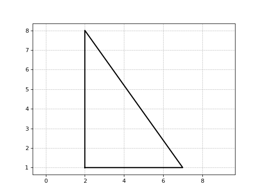
Method for show a graphic of the triangle object.

Returns:object associated with a matplotlib graphic. Return type:ax (matplotlib.axes._subplots.AxesSubplot)

Examples

>>> from numpy import array
>>> from circpacker.basegeom import Triangle
>>> coords = array([(1, 1), (4, 8), (8, 5)])
>>> triangle = Triangle(coords)
>>> triangle.plot()

(Source code, png, hires.png, pdf)

class circpacker.basegeom.Polygon(coordinates)

Bases: object

Creates an instance of an object that defines a Polygon once the cartesian coordinates of its vertices are given.

coordinates

Coordinates of the vertices of the polygon.

Type:(n, 2) numpy.ndarray

area()

Method for determine the area of the polygon.

Returns:area of the polygon surface. Return type:area (float)

Examples

>>> from numpy import array
>>> from circpacker.basegeom import Polygon
>>> coords = array([(1, 1), (4, 8), (8, 5)])
>>> polygon = Polygon(coords)
>>> polygon.area
18.5

>>> from numpy import array
>>> from circpacker.basegeom import Polygon
>>> coords = array([[1, 1], [2, 5], [4.5, 6], [8, 3],
                    [7, 1], [4, 0]])
>>> polygon = Polygon(coords)
>>> polygon.area
27.5

plot()

Method for show the graph of the polygon.

Examples

(Source code, png, hires.png, pdf)

circpacker.packer module

Module to define particular circular tangents in a closed polygon in \(\mathbb{R}^2\).

class circpacker.packer.CircPacking(coordinates, minAngle=None, maxArea=None, length=None, depth=None)

Bases: object

Creates an instance of an object that defines circular particles tangent in a fractal way inside of a closed polygon in \(\mathbb{R}^2\).

coordinates

Coordinates of vertices of the polygon.

Type:(n, 2) numpy.ndarray

depth

Depth fractal for each triangle that compose the triangular mesh. Large values of depth might produce internal variables that tend to infinite, then a ValueError is produced with a warning message array must not contain infs or            NaNs.

Type:int

minAngle

Minimum angle for each triangle of the Delaunay triangulation.

Type:int or float

maxArea

Maximum area for each triangle of the Delaunay triangulation.

Type:int or float

length

Characteristic length This variable is used to model bimsoils/bimrock. The default value is None.

Type:int or float

Note

The class CircPacking requires NumPy, Matplotlib and Triangle

Examples

>>> from numpy import array
>>> from circpacker.packer import CircPacking as cp
>>> coords = array([[1, 1], [2, 5], [4.5, 6], [8, 3], [7, 1], [4, 0]])
>>> pckCircles = cp(coords, depth=5)
>>> pckCircles.__dict__.keys()
dict_keys(['coordinates', 'minAngle', 'maxArea', 'lenght', 'depth',
           'CDT', 'listCirc'])

triMesh()

Method to generate a triangles mesh in a polygon by using Constrained Delaunay triangulation.

Returns:Vertices of each triangle that compose the triangular mesh. n means the number of triangles; (3, 2) means the index vertices and the coordinates (x, y) respectively. Return type:verts ((n, 3, 2) numpy.ndarray)

Examples

>>> from numpy import array
>>> from circpacker.basegeom import Polygon
>>> from circpacker.packer import CircPacking as cp
>>> coordinates = array([[1, 1], [2, 5], [4.5, 6], [6, 4], [8, 3],
                         [7, 1], [4.5, 1], [4, 0]])
>>> polygon = Polygon(coordinates)
>>> boundCoords = polygon.boundCoords
>>> circPack = cp(boundCoords, depth=8)
>>> verts = circPack.triMesh()

>>> from numpy import array
>>> from circpacker.basegeom import Polygon
>>> from circpacker.packer import CircPacking as cp
>>> coordinates = array([[2, 2], [2, 6], [8, 6], [8, 2]])
>>> polygon = Polygon(coordinates)
>>> boundCoords= polygon.boundCoords
>>> circPack = cp(boundCoords, depth=3)
>>> verts =  circPack.triMesh()

generator()

Method to generate circular particles in each triangle of the triangular mesh.

Returns:list that contain all the circles object packed in the polygon. Return type:listCirc (list of Circle objects)

Examples

>>> from numpy import array
>>> from circpacker.packer import CircPacking as cp
>>> coords = array([[2, 2], [2, 6], [8, 6], [8, 2]])
>>> circPack = cp(coords, depth=4)
>>> lstCircles = circPack.generator() # list of circles

plot(plotTriMesh=False)

Method for show a graphic of the circles generated within of the polyhon.

Parameters:plotTriMesh (bool) – Variable to check if it also want to show the graph of the triangles mesh. The default value is False

Examples

(Source code)

>>> from numpy import array
>>> from circpacker.basegeom import Polygon
>>> from circpacker.packer import CircPacking as cp
>>> coordinates = array([[1, 1], [2, 5], [4.5, 6], [6, 4], [8, 3],
                         [7, 1], [4.5, 1], [4, 0]])
>>> polygon = Polygon(coordinates)
>>> boundCoords = polygon.boundCoords
>>> pckCircles = cp(boundCoords, depth=8)
>>> pckCircles.plot()

>>> from circpacker.slopegeometry import AnthropicSlope
>>> from circpacker.packer import CircPacking as cp
>>> slopeGeometry = AnthropicSlope(12, [1, 1.5], 10, 10)
>>> boundCoords = slopeGeometry.boundCoords
>>> pckCircles = cp(boundCoords, depth=3)
>>> pckCircles.plot(plotTriMesh=True)

(Source code)

frecHist()

Method to show the histogram of the diameters of the circular particles packed in a closed polygon in \(\mathbb{R}^2\).

Examples

(Source code, png, hires.png, pdf)

logDiagram()

Method to show the log-log graph of the diameters and quantities of circular particles packed in a closed polygon in \(\mathbb{R}^2\).

Examples

(Source code, png, hires.png, pdf)

circpacker.slopegeometry module

Module for defining the class related to the slope geometry.

class circpacker.slopegeometry.AnthropicSlope(slopeHeight, slopeDip, crownDist, toeDist, maxDepth=None)

Bases: object

Creates an instance of an object that defines the geometrical frame of the slope to perform the analysis.

The geometry of the slope is as follow:

• It is a right slope, i.e. its face points to the right side.
• Crown and toe planes are horizontal.
• The face of the slope is continuous, ie, it has not berms.

slopeHeight

Height of the slope, ie, vertical length betwen crown and toe planes.

Type:int or float

slopeDip

Both horizontal and vertical components of the slope inclination given in that order.

Type:(2, ) tuple, list or numpy.ndarray

crownDist

Length of the horizontal plane in the crown of the slope.

Type:int or float

toeDist

Length of the horizontal plane in the toe of the slope.

Type:int or float

maxDepth

Length of the maximum depth the slope can reach.

Type:int or float or None

Note

The class slopegeometry requires NumPy and Matplotlib.

Examples

>>> slopeGeometry = AnthropicSlope(12, [1, 1.5], 10, 10)
>>> slopeGeometry.__dict__.keys()
dict_keys(['slopeHeight', 'slopeDip', 'crownDist', 'toeDist',
           'maxDepth', 'boundCoords'])

maxDepth()

Method to obtain the maximum depth of a slope where a circular slope failure analysis can be performed.

The maximum depth is such that the biggest circle satisfished the following conditions:

• It is tangent to the bottom.
• crosses both the extreme points at the crown and toe.
• It is orthogonal to the crown plane.

Returns:Maximum depth of the slope measured vertically from the toe plane. Return type:maxDepth (int or float)

Examples

>>> slopeGeometry = AnthropicSlope(12, [1, 1.5], 10, 10)
>>> slopeGeometry.maxDepth()
4.571428571428573

defineBoundary()

Method to obtain the coordinates of the boundary vertices of the slope and plot it if it is wanted.

The origin of the coordinates is in the corner of the bottom with the back of the slope. The coordinates define a close polygon, ie, the first pair of coordinates is the same than the last one.

Returns:Coordinates of the boundary vertices of the slope. Return type:(numpy.ndarray)

Examples

>>> slopeGeometry = AnthropicSlope(12, [1, 1.5], 10, 10)
>>> slopeGeometry.defineBoundary()
array([[  0.        ,   0.        ],
       [ 28.        ,   0.        ],
       [ 28.        ,   4.57142857],
       [ 18.        ,   4.57142857],
       [ 10.        ,  16.57142857],
       [  0.        ,  16.57142857],
       [  0.        ,   0.        ]])

plotSlope()

Method for generating a graphic of the slope boundary.

Examples

>>> slopeGeometry = AnthropicSlope(12, [1, 1.5], 10, 10)
>>> slopeGeometry.plotSlope()

(Source code, png, hires.png, pdf)

class circpacker.slopegeometry.NaturalSlope(surfaceCoords)

Bases: object

Creates an instance of an object that defines the geometrical frame of the slope to perform the analysis.

The geometry of the slope is as follow:

• It is a right slope, i.e. its face points to the right side.
• The slope is defined with its surface’s coordinates.
• The surface is defined as a polyline such that each segment’s slope are always zero or negative.
• The coordinates’ order is such that the highest (and leftmost) point is the first one, and the lowest (and rightmost) is the last one.

surfaceCoords

Coordinates of the surface’s vertices of the slope.

Type:numpy.ndarray

Note

The class NaturalSlope requires NumPy and Matplotlib.

Examples

>>> from numpy import array
>>> surfaceCoords = array([[  0.        ,  16.57142857],
                           [ 10.        ,  16.57142857],
                           [ 18.        ,   4.57142857],
                           [ 28.        ,   4.57142857],
                           [ 28.        ,   0.        ]])
>>> slopeGeometry = NaturalSlope(surfaceCoords)
>>> slopeGeometry.__dict__.keys()
dict_keys(['surfaceCoords', 'slopeHeight', 'maxDepth', 'boundCoords'])

maxDepth()

Method to obtain the maximum depth of a slope where a circular slope failure analysis can be performed.

The maximum depth is such that the biggest circle satisfished the following conditions:

• It is tangent to the bottom.
• crosses both the extreme points at the crown and toe.
• It is orthogonal to the crown plane.

Returns:Maximum depth of the slope measured vertically from the toe plane. Return type:maxDepth (int or float)

Examples

>>> from numpy import array
>>> surfaceCoords = array([[  0.        ,  16.57142857],
                           [ 10.        ,  16.57142857],
                           [ 18.        ,   4.57142857],
                           [ 28.        ,   4.57142857]])
>>> slopeGeometry = NaturalSlope(surfaceCoords)
>>> slopeGeometry.maxDepth()
4.571428571428573

defineBoundary()

Method to obtain the coordinates of the boundary vertices of the slope and plot it if it is wanted.

The origin of the coordinates is in the corner of the bottom with the back of the slope. The coordinates define a close polygon, ie, the first pair of coordinates is the same than the last one.

Returns:Coordinates of the boundary vertices of the slope. Return type:(numpy.ndarray)

Examples

>>> from numpy import array
>>> surfaceCoords = array([[  0.        ,  16.57142857],
                           [ 10.        ,  16.57142857],
                           [ 18.        ,   4.57142857],
                           [ 28.        ,   4.57142857]])
>>> slopeGeometry = NaturalSlope(surfaceCoords)
>>> slopeGeometry.defineBoundary()
array([[  0.        ,   0.        ],
       [  0.        ,  16.57142857],
       [ 10.        ,  16.57142857],
       [ 18.        ,   4.57142857],
       [ 28.        ,   4.57142857],
       [ 28.        ,   0.        ],
       [  0.        ,   0.        ]])

>>> from numpy import array
>>> surfaceCoords = array([[-2.4900, 18.1614],
                           [0.1022, 17.8824],
                           [1.6975, 17.2845],
                           [3.8909, 15.7301],
                           [5.8963, 14.3090],
                           [8.1183, 13.5779],
                           [9.8663, 13.0027],
                           [13.2865, 3.6058],
                           [20.2865, 3.6058],
                           [21.4347, 3.3231],
                           [22.2823, 2.7114],
                           [23.4751, 2.2252],
                           [24.6522, 1.2056],
                           [25.1701, 0.2488]])
>>> slopeGeometry = NaturalSlope(surfaceCoords)
>>> slopeGeometry.defineBoundary()
array([[  0.00000000e+00,   0.00000000e+00],
       [  0.00000000e+00,   1.96301237e+01],
       [  2.59220000e+00,   1.93511237e+01],
       [  4.18750000e+00,   1.87532237e+01],
       [  6.38090000e+00,   1.71988237e+01],
       [  8.38630000e+00,   1.57777237e+01],
       [  1.06083000e+01,   1.50466237e+01],
       [  1.23563000e+01,   1.44714237e+01],
       [  1.57765000e+01,   5.07452373e+00],
       [  2.27765000e+01,   5.07452373e+00],
       [  2.39247000e+01,   4.79182373e+00],
       [  2.47723000e+01,   4.18012373e+00],
       [  2.59651000e+01,   3.69392373e+00],
       [  2.71422000e+01,   2.67432373e+00],
       [  2.76601000e+01,   1.71752373e+00],
       [  2.76601000e+01,   6.66133815e-16],
       [  0.00000000e+00,   0.00000000e+00]])

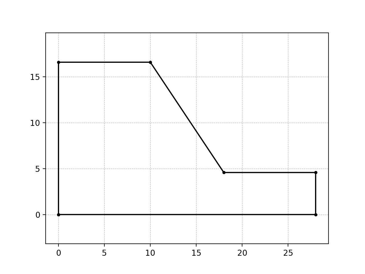
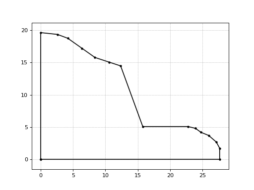
plotSlope()

Method for generating a graphic of the slope boundary.

Examples

>>> from numpy import array
>>> surfaceCoords = array([[  0.        ,  16.57142857],
                           [ 10.        ,  16.57142857],
                           [ 18.        ,   4.57142857],
                           [ 28.        ,   4.57142857]])
>>> slopeGeometry = NaturalSlope(surfaceCoords)
>>> slopeGeometry.plotSlope()

(Source code, png, hires.png, pdf)

>>> from numpy import array
>>> surfaceCoords = array([[-2.4900, 18.1614],
                           [0.1022, 17.8824],
                           [1.6975, 17.2845],
                           [3.8909, 15.7301],
                           [5.8963, 14.3090],
                           [8.1183, 13.5779],
                           [9.8663, 13.0027],
                           [13.2865, 3.6058],
                           [20.2865, 3.6058],
                           [21.4347, 3.3231],
                           [22.2823, 2.7114],
                           [23.4751, 2.2252],
                           [24.6522, 1.2056],
                           [25.1701, 0.2488]])
>>> slopeGeometry = NaturalSlope(surfaceCoords)
>>> slopeGeometry.plotSlope()

(Source code, png, hires.png, pdf)

Module contents

Top-level package for CircPacker.